 Català (Catalan)
  Español (Spanish)
It has been some time since I last wrote an article that was a bit technical and not at all pedagogical. Today I want to talk about the conditional formatting of Google spreadsheets. Recovering a functionality of my gradebook I have found this casuistry and, if you don’t know it, maybe it can be useful for you.
As most of you know, conditional formatting in spreadsheets, as the name suggests, allows the formatting of a cell to change if certain conditions occur. For example, we can make a cell with a number appear red if it is negative or black if it is positive. What I want to show in this article is how to change the format of a cell based on the values we enter in another cell that is also in another tab of the same spreadsheet (or better said, in another sheet of the same spreadsheet).
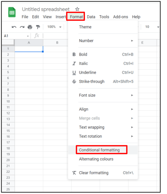
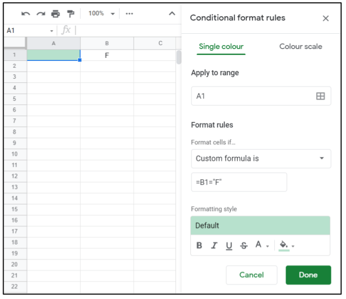
There are many conditional formatting options: if the cell is empty, if there is a number, if the number is less or greater than a quantity, if it contains text, etc. But they all refer to the same cell where we apply it. If we want the format to change from the content of a different cell, we have to use the last option of all, custom formula.
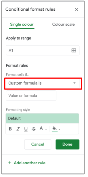
This formula will always start with an equal. For example, we can put
=B1="F"
Now, our current cell, let’s say A1, will change format when we enter the value F in cell B1.
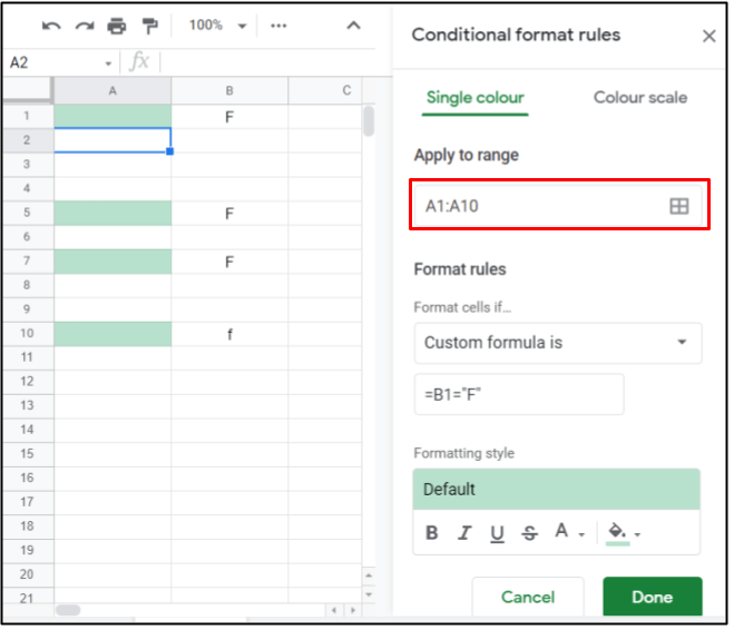
In addition, we could make this conditional formatting take effect on a range of cells, not just cell A1. For example, it could take effect in the range A1: A10. To achieve this, we have two options. Either we copy and paste (with the paste conditional formatting only option) or we simply indicate the range A1: A10 in the box where it says Apply to range.
Although we won’t see it anywhere, as the formula has no $ sign, the cell reference changes in the other cells of the range. In cell A2, it is as if the conditional formatting had the formula = B2 = “F”, although if we look at the conditional formatting, it still indicates the formula with respect to B1.
So far, so good, but what happens if we want the cell containing the value that produces the formatting change to be on another sheet? It would be logical to think that you just have to indicate the cell with the name of the sheet. For example, = ‘Sheet 2’! B1 = “F”.
It may be very logical, but it doesn’t work. To make it work, we need to use another formula, the INDIRECT formula. So, we should write,
=INDIRECT("'Sheet 2'!B1")="F"
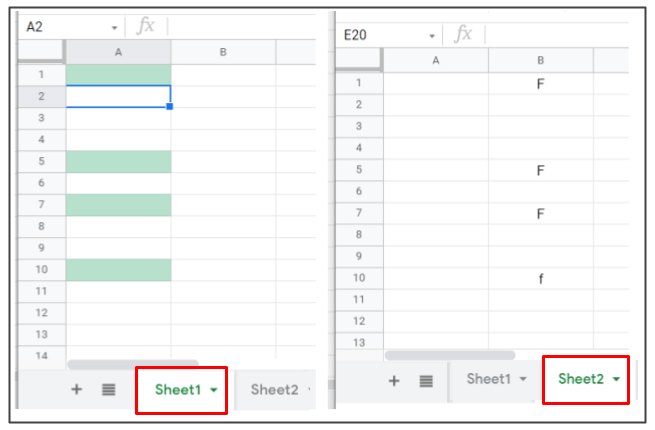
It doesn’t seem so complicated, does it? But, as always in these things, there are side effects and it doesn’t work well. Note that now the reference to cell B1 is inside a text field (it is in inverted commas). Therefore, the spreadsheet does not interpret it as a reference to a cell but as a text. And what is the consequence of this? It only works well in cell A1. In the others, even if there is no dollar sign, it does not work. When in cell ‘Sheet 2’! B1 you put an F, the whole range A1: A10 changes colour. When it is left blank or any other value is entered, the whole range A1: A10 loses its colour.
Is there a solution? Yes, of course there is. Just make the formula a bit more complicated so that the reference to B1 is not in a text field.
=INDIRECT("'Sheet 2'!"&ADDRESS(ROW(A1);COLUMN(A1)+1))="F"
Inside the INDIRECT formula, from the text field, we put the formula ADDRESS, which will create a reference to a cell, from indicating a row number and a column number.
As a row, we will indicate the same of our cell A1, therefore, ROW (A1). And as a column, one more than the one in our cell A1, since on sheet 2 we are looking at column B.
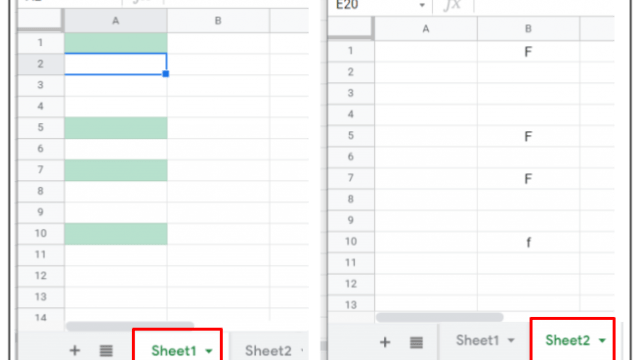
In this way, the references to A1 are references to cells and are not text fields. Therefore, when applied to the range, they will be updated and the conditional formatting will work correctly.