 Català (Catalan)
  Español (Spanish)
Lately I have been asked several times how to perform this operation. Several teachers have classes with the same students (although not exactly the same) and all evaluate the same aspects. Each one has their own sheet with their students and they want to be able to gather all the information and make averages. In addition, you can also create one sheet per student so that they can only see their results.
In this article I will detail a possible way to do it.
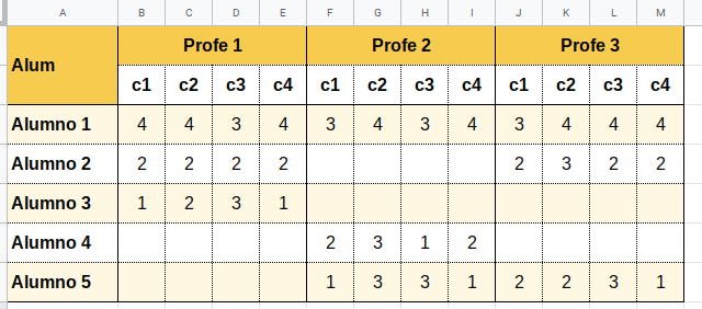
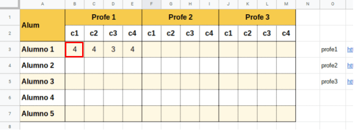
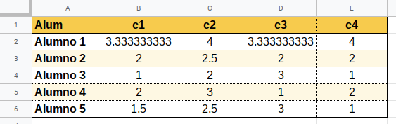
Let’s start with each teacher’s sheet. To make it simple, in the example I will suppose only 3 teachers who evaluate 5 students (although each one only evaluates 3) and each one registers 4 different aspects.
The sheet of one of the teachers could be as follows (in the example each aspect is scored between 1 and 4). In order to do tests it is good that values have been introduced, so it is easy to see if they are imported well.
The general sheet could be as follows.
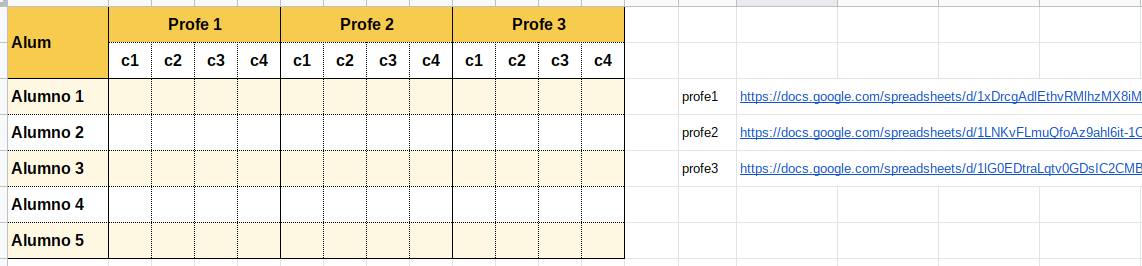
At the moment the sheet does not collect anything, but the addresses of the 3 sheets of teachers have already been indicated.
What formula should be used so that each student’s grades appear?
We will use the IMPORTRANGE formula (which I presented in an article some time ago). But first we will have to connect the sheets, because if this is not done, the importrange formula combined with other formulas will not work.
Therefore, in any cell (in the example I use B3), we insert the following formula (which we will delete later).
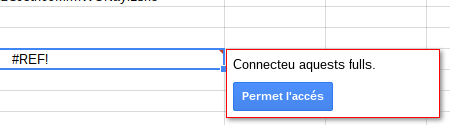
=IMPORTRANGE(P3;”Sheet1!B3″)
Surely, an error will appear to us (I do not know why, in some occasions the sheets have been connected to me without asking for permission). When we put the cursor over the cell, the message will appear to give permission and connect the sheets.
Once the first sheet is connected, we will change the formula to connect the second sheet. Now we will indicate
=IMPORTRANGE(P3;”Sheet1!B3″)
And we’d do that with all the leaves. Once they were all connected, we would eliminate the formula.
Now, we will introduce the formula so that it collects the data of each student. In cell B3 we will indicate the following formula.
=FILTER(IMPORTRANGE($P$3;”Sheet1!B3:E5″);IMPORTRANGE($P$3;”Sheet1!A3:A5″)=$A3)
If we want to avoid errors in case the student is not in the teacher’s sheet, we can add the formula IFERROR. It would look like this.
=IFERROR(FILTER(IMPORTRANGE($P$3;”Sheet1!B3:E5″);IMPORTRANGE($P$3;”Sheet1!A3:A5″)=$A3);””)
We can now copy the formula to the rest of the students.
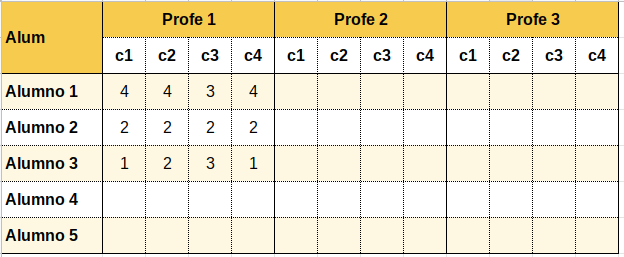
Only the grades of the students who were on the teacher’s sheet appear.
We can do the same with the sheets of the other teachers. In cell F3 we will indicate the same formula that we have inserted in B3, but changing $P$3 for $P$4 that is where the direction of the sheet of the second teacher is indicated.
=IFERROR(FILTER(IMPORTRANGE($P$4;“Sheet1!B3:E5”);IMPORTRANGE($P$4;“Sheet1!A3:A5”)=$A3);“”)
Y también la copiaremos a todos los alumnos.
Repetimos el procedimiento con la tercera hoja de profesor.
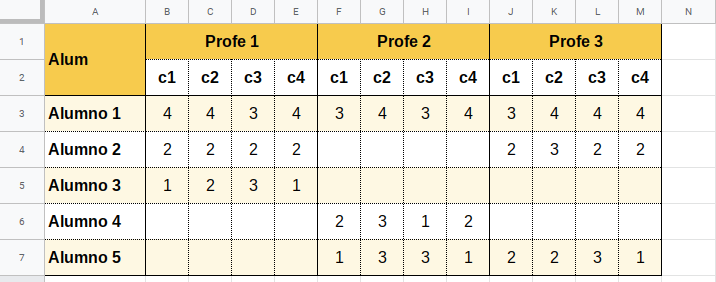
Any changes a teacher makes to your sheet will be reflected in this summary sheet.
Calculating the average will be more or less straightforward. We can create a new tab and sort it as follows.
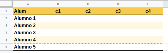
In cell B2 we can indicate the following formula.
=AVERAGEIF(Sheet1!$B$2:$M$7;B$1;Sheet1!$B3:$M3)
This will display the average of the teachers who have indicated this aspect.
Just copy this formula to the rest of the cells (from B2 to E6) and you will have all the averages calculated.
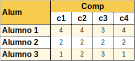
Results sheet for each student
Can we have each student see their results? We’ll have to create a spreadsheet for each student and share it with read-only permission (it can be done with a script, but in the title I said everything would be without scripts, so we’ll do it manually). But let’s start with the first student’s sheet.
The sheet may look like the following.
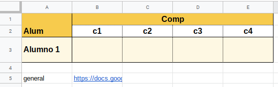
As you can see, you have to indicate the direction of the summary sheet, where the results will be. To avoid students trying to access and ask for permission (since they do not have permission to read on the summary sheet), I would hide row 5.
As we have done before, you have to connect the sheets. In cell B3 we introduce the simple importrange formula.
=IMPORTRANGE(B5;”Sheet1!B3″)
Once connected, we delete the formula and enter the following one.
=FILTER(IMPORTRANGE($B$5;”Sheet2!B2:E6″);IMPORTRANGE($B$5;”Sheet2!A2:A6″)=$A3)
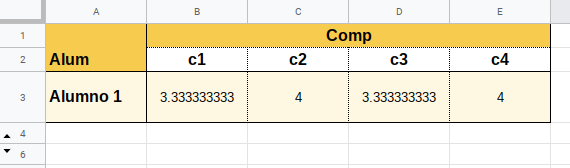
Now all you have to do is make a copy of this sheet and change cell A3. If we put Pupil 2, the results of the second pupil will appear. It’s that simple.
Templates
Here I link the templates of the example, in case someone wants to make a copy. In order for it to work you will have to change the links, since the copies will have other addresses.
