 Català (Catalan)
  Español (Spanish)
I sincerely believe that spreadsheets are one of the most useful tools for teachers. I have said it more than once and, for me, should be one of the digital skills of a teacher. It’s true that I haven’t dedicated much time to them in this blog. A couple of years ago I dedicated one to the IMPORTRANGE formula. Today I will talk about another formula that can also be very useful, ARRAYFORMULA. It is especially useful when working with spreadsheets that collect responses from Google forms.
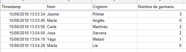
Let’s imagine that we want to have a spreadsheet with some information about the students (name, surname, number of siblings…). With Google forms it’s very simple. We create the form, send the link to the students and they reply themselves.

Once the students have answered, we can open the form in edit mode and, in the Responses section, we can create the spreadsheet.

A spreadsheet will be opened with all the students’ answers.
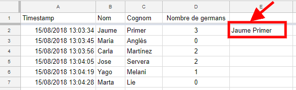
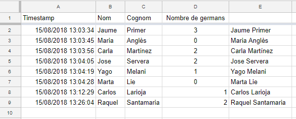
Let us now suppose that we want to work a little with this data. For example, we want to do something as simple as adding a field where the first and last names are together. Let’s go to the first free column and use the following formula:
=B2 & ” ” & C2
In fact, the name and surname appear in a single cell.
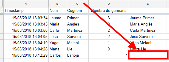
If we want this field to be for all students, we will have to copy the formula to all students. No problem at all.
But what happens if a student answers the form late? One might think that it is enough to copy the formula into the entire E column and then we have it ready for any number of answers. But that is not the case.
When a form is answered, Google inserts a new row at the end of the last answer and therefore does not respect any formula (or format) that we had foreseen. If the form is answered after you have copied the formula, it will appear as follows.
How can we do it to have the sheet ready and when the students answer the question, we don’t have to copy formulas?
One option is to use a spreadsheet add-on called copyDown. It is an option, but in many cases, there is a simpler solution. Use the formula ARRAYFORMULA.
This formula converts a formula that returns one value (in our case the first and last names together) into a formula that returns many values. In other words, with a single formula in the first student, we will have the field for everyone.
Just put in the following formula:
=ARRAYFORMULA(B2:B & ” ” & C2:C)
You can see that the formula is the same as the one we entered, but changing the values (B2 and C2) to the ranges (B2: B and C2: C). The ARRAYFORMULA formula tells the sheet to take all the values in range B2: B (from B2 to the end of column B2) and apply the formula.
To make it work for us, we will have to delete the formulas we had copied, otherwise the sheet will complain that the cells will be overwritten.
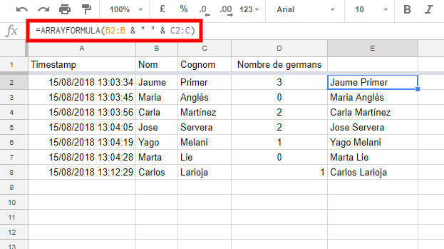
In this version, there is only one formula in cell E2. Therefore, if the form is now answered, it will not be necessary to touch anything and everything will continue to work.
Even if forms are not used, the formula is also very useful to save us work. With a single formula it works for us, without having to copy and paste formulas.
For advanced users, this formula can be combined with other COUNTIF, AVERAGE, VLOOKUP, IMPORTRANGE… However, it is not compatible with all of them. For example, it does not work with FILTER or QUERY.
